Newton's method provides a numerical solution to the roots of any equation, and the optimization problem is generally converted into finding the distance between functions in a "normed linear space"minimum point, so, use Newton’s method to solve any objective functionextreme pointIt's a good idea.

Equation finding roots

For a quadratic equation of one variable, finding the root is actually very simple. Just apply the root formula. However, finding the root formula of an equation (Analytical solution) is actually very difficult. It can be proved that there is no analytical solution for equations of degree 5 or above. Other complex equations such as partial differential equations are even more difficult to solve. Fortunately, with the development of computer technology, analytical solutions are no longer so important (at least in engineering), and the replacement method is numerical solution.Newton's methodIt is one of many numerical solutions.
Numerical solution is also called numerical analysis. It mainly uses the idea of approximation to make the numerical solution continue to approach the analytical solution through iterative calculations, and the solution obtained is calledNumerical solution, in engineering, numerical solutions are useful as long as they satisfy the equation within the accuracy requirements.

Newton's iteration method

$ASIC Flow$

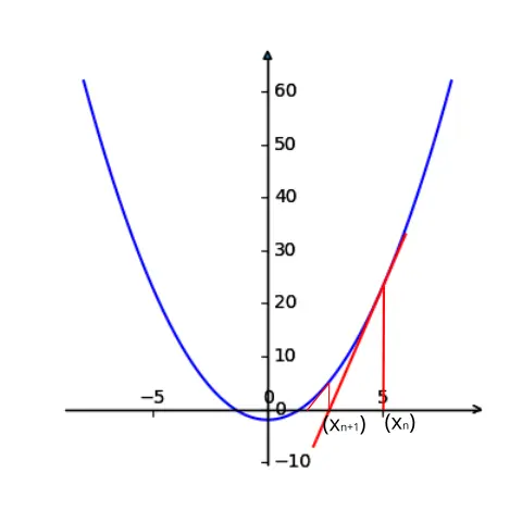
Figure 1 Newton iteration method

sqrt2.png

Let’s consider a small problem first: solving the equation $x^2-2=0$ The root of , that is, solving $qrt 2$ . The idea of Newton's iteration method is easy to understand from a geometric point of view, as shown in the figure above (the script for drawing is inhereopen in new window) The root of the equation is the function $y=x^2-2$ with $x$ The value of the abscissa at the intersection of the axes. from the picture $x_n$ Starting from the point, the calculation function is $x_n$ tangent line at the point, and then calculate the tangent line sum $x$ The intersection point of the axes is obtained $x_{n+1}$ , and then calculate the function in $x_{n+1}$ The tangent line at the point... Keep iterating like this, you can find $x_{n}$ will get closer and closer to the roots of the equation.

Mathematical expression of the above idea:
by $x_{n}$ Calculate $y_{n}$

Get the tangent equation:

y-y_n= eft. f(x)' ight | _{x=x_n}(x-x_n) — y-y_n= \left. f(x)' \right | _{x=x_n}(x-x_n)

tangent sum $x$ The intersection point of the axes, that is, when $y=0$ when,

0-y_n=eft. f(x)' ight | _{x=x_n}(x-x_n) — 0-y_n=\left. f(x)' \right | _{x=x_n}(x-x_n)

rac{-y_n}{eft. f'(x) ight | _{x=x_n}} = (x-x_n) — \frac{-y_n}{\left. f'(x) \right | _{x=x_n}} = (x-x_n)

when $eft. f'(x) ight | _{x=x_n} eq 0$ when,

x = x_n- rac{y_n}{eft. f'(x) ight | _{x=x_n}} — x = x_n- \frac{y_n}{\left. f'(x) \right | _{x=x_n}}

by $y_n = f(x_n)$ , get:

x = x_n- rac{f(x_n)}{eft. f'(x) ight | _{x=x_n}} — x = x_n- \frac{f(x_n)}{\left. f'(x) \right | _{x=x_n}}

Order $x=x_n$ , continue to iterate, and you will get the iteration formula:

x_{n+1} = x_n- rac{f(x_n)}{eft. f'(x) ight | _{x=x_n}} — x_{n+1} = x_n- \frac{f(x_n)}{\left. f'(x) \right | _{x=x_n}}

The derivation process can also be derived fromThe angle of the Taylor expansion of the functionTo understand, this has been written in many blogs, so I won’t go into details here.

According to the above iteration formula, the equation can be calculated $x^2-2=0$ The roots are:

Guess an initial value, because the root is probably more than 1 o'clock, then give it $x_0=2$ Okay;
Calculate $x_1$ ：
$x_{1} = x_0- rac{f(x_0)}{eft. f'(x) ight | _{x=x_0}}= 2- rac{f(2)}{eft. f'(x) ight | _{x=2}}=1.5$
$x_{2} = 1.5- rac{f(1.5)}{eft. f'(x) ight | _{x=1.5}}=1.416667$
$x_{3} = 1.416667- rac{f(1.416667)}{eft. f'(x) ight | _{x=1.416667}}=1.414216$

Analysis of algorithm advantages and disadvantages

The advantage of Newton's method is of course that it provides a numerical solution method for finding the roots of equations. There are also several disadvantages:

First of all, the algorithm requires that the function be differentiable everywhere. If the derivative function needs to be continuous for the optimization problem (because second-order derivatives are required everywhere), otherwise the algorithm cannot calculate the roots of the function, such as $f(x)=x^{1/3}$ It cannot converge. Although the root of the function is 0, its derivative at 0 does not exist;
The solution obtained may be only one of many solutions. This comparisonDepends on the selection of initial values, for example, in the above problem, if the initial value is 2, it will converge to the positive solution of the equation. If you want to get a negative solution, you need to choose the initial value among negative numbers. For real-life problems, it is difficult to estimate the size range of the solution;
If the initial estimate is too far away from the root, convergence will become slower;
It is required that the tangent derivative obtained in each iteration cannot be 0, as shown in the derivation process;
If the equation has no roots, Newton's method cannot converge;

Optimization problem solving

The optimization problem is understood from a functional perspective, which is to calculate the minimum distance between functions. There are many definitions of distance, the more commonly used ones aresecond norm, makesecond normThe solution process for minimizing distance is called least squares. for $Gm=data_{predict}$ For such a linear problem (non-threaded problems can be converted into linear problems through Taylor expansion), the distance can be defined as $hi (m)=||Gm-data_{observation}||_2$ , in order to find the minimum distance point, we need to find the extreme point first, and the problem is converted into a solution $hi '(m)=0$ roots, at this timeNewton's methodIt came in handy. Different from the previous question, here it is required $hi '(m)$ The derivative of , that is, solving $hi "(m)$ , that is, the Hessian matrix. Assume that the parameters here $m$ is an n-dimensional vector, then the Hessian matrix is:

H = egin{pmatrix} rac{artial ^2f}{artial m_1^2} & rac{artial ^2f}{artial m_1 artial m_2} & dots & rac{artial ^2f}{artial m_1 artial m_n} rac{artial ^2f}{artial m_2 artial m_1} & rac{artial ^2f}{artial m_2^2} & dots & rac{artial ^2f}{artial m_2 artial m_n} dots & dots & dots & dots rac{artial ^2f}{artial m_n artial m_1} & rac{artial ^2f}{artial m_n artial m_2} & dots & rac{artial ^2f}{artial m_n^2} nd{pmatrix} — H = \begin{pmatrix} \frac{\partial ^2f}{\partial m_1^2} & \frac{\partial ^2f}{\partial m_1 \partial m_2} & \cdots & \frac{\partial ^2f}{\partial m_1 \partial m_n} \ \frac{\partial ^2f}{\partial m_2 \partial m_1} & \frac{\partial ^2f}{\partial m_2^2} & \cdots & \frac{\partial ^2f}{\partial m_2 \partial m_n} \ \vdots & \vdots & \ddots & \vdots \ \frac{\partial ^2f}{\partial m_n \partial m_1} & \frac{\partial ^2f}{\partial m_n \partial m_2} & \cdots & \frac{\partial ^2f}{\partial m_n^2} \ \end

Therefore, to solve the optimization problem using Newton's method, you need to first find the Jacobian matrix and the Hessian matrix of the objective function. The most computationally intensive part is calculating the Hessian matrix, because the amount of second-order derivative calculation increases exponentially.

Note that if the second derivative here is continuous, then $H$ is a symmetric matrix.

Algorithm steps

Step 1: Given error threshold $0eqpsilon <<1$ , initial model $m_0$ (The number of iterations can also be given);
Step 2: Calculate gradient $g_k=abla f(m_k)$ , if $g_keq psilon$ , stop calculation, output $m^* pprox m_k$ ;
Step 3: Calculate Hessian matrix $G_k=abla^2f(m_k)$ , calculate $d_k=rac {g_k}{G_k}$ ;
Step 4: order $x_{k+1}=x_{k}-d_{k}$ , k=k+1, go to step 2.

Example

An example: finding the minimum value $f(m_1,m_2) = -m_13-m_23+3m_12+2m_22+m_1+m_2-1$

#include <stdio.h>
#include <math.h> double funY(double x);
double funY1(double x); int main() { double x, x1, x2; x1 = 1.5;//Find the roots near 1.5 x2 = x1 - funY(x1) / funY1(x1); while (fabs(x2 - x1) > 1e-6) { x1 = x2; x2 = x2 = x1 - funY(x1) / funY1(x1); } printf("%lf",x2);
}
//————————————————————
// function of y
double funY(double x) { double y; y = 2 * x*x*x - 4 * x*x + 3 * x - 6; return y;
}
//The first derivative of y
double funY1(double x) { double y1; y1 = 6 * x*x - 8 * x + 3; return y1;
}

Several ways to improve

The key considerations for optimization calculations include the versatility, effectiveness, convergence, and efficiency of the algorithm. Of course, these are included in the time complexity and space complexity. There are several issues with Newton's method that need to be considered:

Calculating the Hessian matrix consumes too many resources and time;
Newton's method is unstable, only $H$ Convergence occurs only when positive timing is reached, that is, the Hessian matrix of the objective function is required. $H_{i,j}$ at each iteration point $m_i$ is positive definite, otherwise it would be difficult to guarantee the direction of convergence of Newton’s method. In fact, $H$ Most likely a pathological/singular matrix;
initial model $m_0$ It is very important. If you choose poorly, it will iterate many times and the convergence will be slower;
The selection of the initial model is not near the minimum value, and it is easy for the result to fall into a local minimum.

In this regard, the experts have proposed some improvement methods:

Quasi-Newton method: In order to avoid calculating the Hessian matrix, do not calculate it directly $H$ , instead construct a matrix $K$ To approximate, $K$ Need all the timeZhengdingandIt’s relatively simple to update, you can view relevant literature here, so I won’t go into details;
Gauss-Newton method: convert the objective function $hi (m)=||Gm-data_{observation}||_2$ Convert to $hi (m)=rac {1}{2}||r(m)||_2$ , among which $r(m)$ Represents the residual, then according to the chain rule, we can get:
$abla^2 hi (m)=abla r(m) abla^T r(m)+um_{i=1}nr_i(m)\nabla2 r_{i}(m)$
order here $Q(m)=um_{i=1}nr_i(m)\nabla2 r_{i}(m)$ , if for the values to be iterated $m^*$ , there is $r_{i}(m^*)=0$ rule $Q(m)=0$ ; In this case, there is no need to calculate the Hessian matrix. This is a good idea, when $m^*$ When the distance to the extreme point/minimum value is relatively close, it is perfect; however, when the initial value is far from the minimum value, $Q(m) pprox 0$ The idea will not work. At this time, the Gauss-Newton method does not converge.

Therefore, the Gauss-Newton method is also extremely dependent on the selection of the initial model/initial value.

Levenberg-Marquardt algorithm: This method combines the Gauss-Newton method and the steepest descent method/gradient method. Because the Gauss-Newton method relies more on the initial model/initial value, the gradient method can overcome this problem; while the convergence speed of the gradient method is slower than the Gauss-Newton method, so this method can provide numerical solutions to numerical nonlinear minimization (local minimum). In fact, the method is very simple, that is, adding a parameter to the objective function $ambda$ , so this method is also called the damped least squares method. A similar approach occurs in Tikhonov regularization.

All these methods may get stuck in local minima instead of finding the global minimum/minimum. To overcome this problem, heuristic/nonlinear optimization algorithms are needed.

Newton iteration

# Equation finding roots

# Newton's iteration method

Figure 1 Newton iteration method

# Analysis of algorithm advantages and disadvantages

# Optimization problem solving

# Algorithm steps

# Example

# Several ways to improve