The line segment connecting x1 and x2 is called a closed line segment if it includes the endpoints of x1 and x2, and it is called an open line segment if it does not. Mathematically expressed as: Take any point x inside the line segment, and if you can write/describe the trajectory of this point x or the law of its coordinate changes,
That's it. In order to do this, we imagine that there are x1,
As shown in the figure below, the general approach is to draw a parallel line of the vector ox2 through the point x. In the triangle in the figure below, there are two blue and one red vectors. The blue vector on the , when the coefficient lamda in front of x1 and x2 changes between 0 and 1, x will also change back and forth on the line segment x1x2, then the trajectory of all x is a closed line segment; if lamda does not take 0 and 1, then it is called an open line segment.
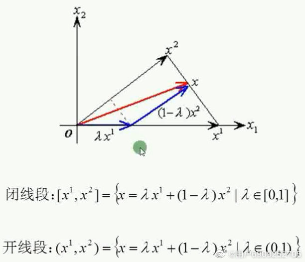
Figure 1 Geometric programming
An example was mentioned before, as shown in the figure below. The intersection points (2,2) and (3,3/2) are both optimal solutions, and any value connecting the two point line segments is the optimal solution; so a closed line segment is just a closed line segment connected with two points as endpoints.
A convex set, like the first figure in the figure below, is a convex polygon, and a region/set enclosed by the polygons that are supplemented/topped is called a convex set.
Mathematically it can be described like this:
If any two points are selected inside a set and the closed line segment connecting the two points is still contained in the set, we call the set a convex set.
Therefore, if there are several such straight lines, the convex polygon area enclosed must represent a convex set.
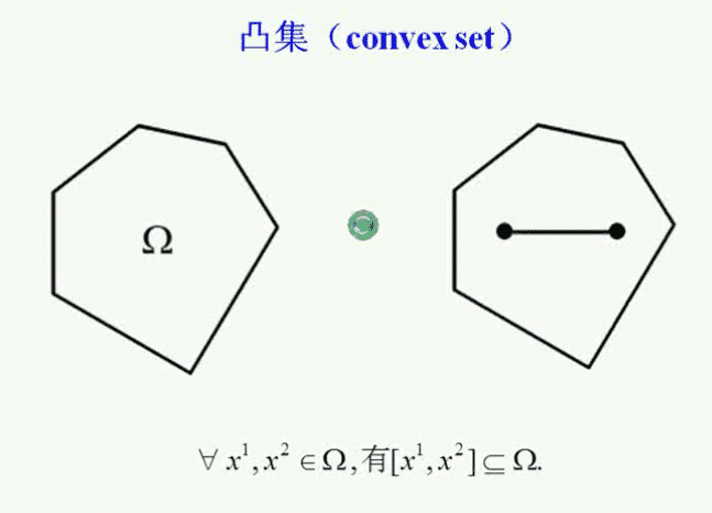
Figure 2 Convex set
Attention everyone: Is the circular surface a convex set? Definitely. Because choose any two points inside it. . . .
However, the circle is not a convex set, because if you pick any two points on the edge of the circle, it is obvious that they are not completely on the circle. In the same way, neither is the sphere. However, a sphere is a convex set.
Vertex: It is a point that is not inside the line connecting any two points (excluding endpoints); the five vertices in the figure below (marked);
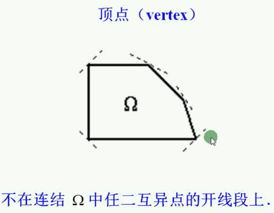
Figure 3 Convex polygon vertices
As can be seen from the above figure, the vertices of convex polygons (which exactly form a convex set) are exactly the vertices of the convex set formed by convex polygons. So, the circular surface is a convex set, so does the circular surface have vertices? Yes, the boundary of a circle is its vertex.
In the same way, the vertex of a sphere represents the surface of the sphere. So don't think that the vertices of a convex set are always the vertices of a convex polygon. This is not necessarily the case. Because this convex set itself does not necessarily represent a polygonal area. Various convex sets have various vertices,
Just like the circles and spheres here they also have their own vertices. My own understanding: that is, the vertices of the convex set can be faces or curves.
Basic theorem of linear programming:
\1. K is a convex set; K is the feasible region (the feasible region of the linear programming problem); that is to say, the feasible region of the linear programming problem is a convex set; look at the figure below, the example we have seen, this example has the only optimal solution, and its feasible region is surrounded by blue line segments, which is obviously a convex set;
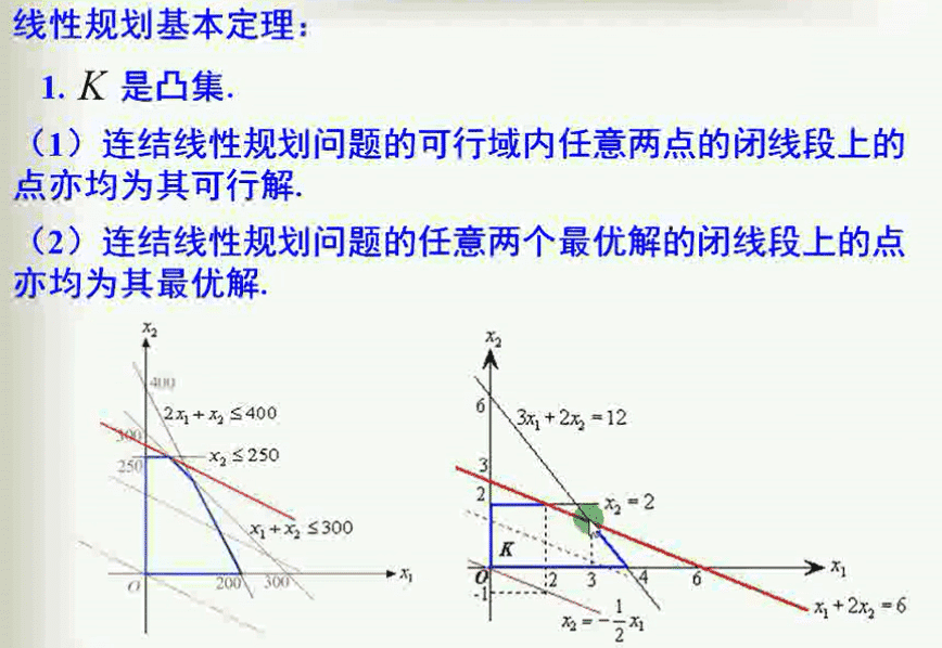
Figure 4 Basic theorem of linear programming
The basic feasible solution of LP is in one-to-one correspondence with the vertices of its feasible region.
As shown in the coordinate diagram below, there are 5 vertices in the feasible region, so the corresponding linear programming problem has 5 basic feasible solutions; because there is a one-to-one correspondence, no more, no less.
The basic feasible solution may not be so intuitive to understand, a bit abstract, and not so easy to understand. But the vertex of the feasible region is very straightforward, it is a geometric point.
In other words, the vertex of the feasible region determines its basic feasible solution, and the two are in one-to-one correspondence.
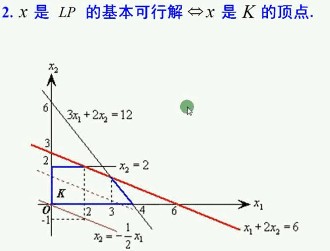
Figure 5 Solution of linear programming
If that feasible region is not the empty set, then it has at least one vertex. If the set is empty, there will be no more.
For example, the example we learned before is an example where the objective function is unbounded. Although its feasible domain is also unbounded, it is not an empty set; unbounded and empty sets are not the same thing. It can also be seen that it has two vertices and is not an empty set; so the conclusion is correct;
If the feasible region is the empty set, then there will be no vertices, as shown in the legend in the lower right corner of the figure below.
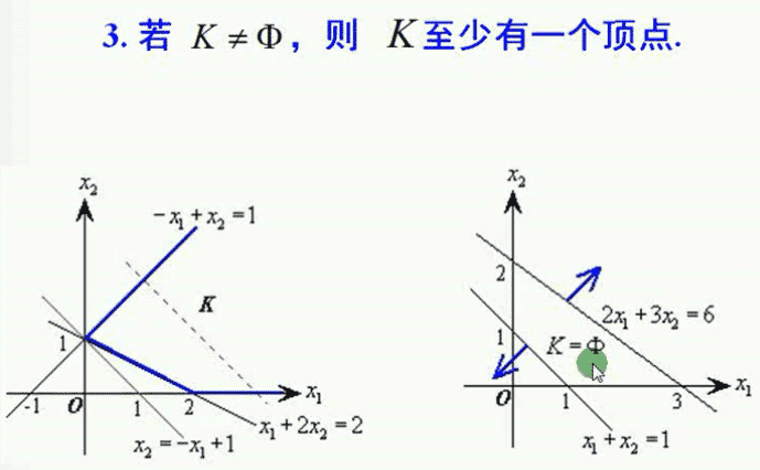
Figure 6 Solution of linear programming
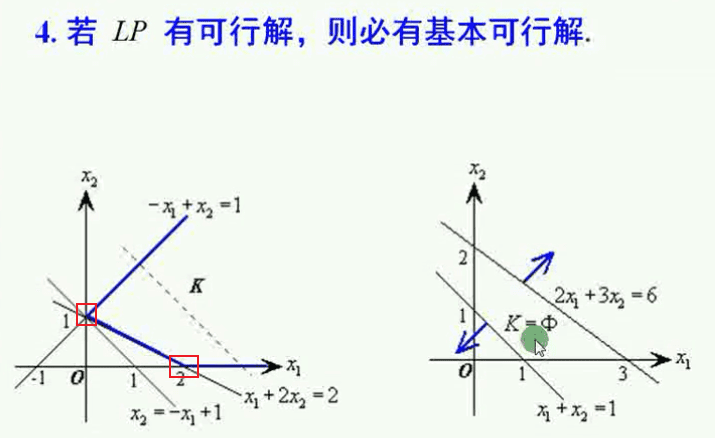
Figure 7 Solution of linear programming
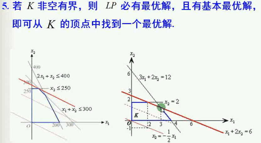
Figure 8 Solution of linear programming
There are at most Cnm vertices in a feasible region, n variables, and m constraints. In the coefficient matrix, m columns are taken from n columns to construct a base, which is the maximum number of possible bases. Of course, there are not necessarily so many, but this is the upper limit.
The number of basic feasible solutions will certainly not exceed the upper limit, but there is no way to find the optimal solution from up to so many basic feasible solutions by enumerating/exhausting the method and comparing the pros and cons one by one. Too slow!
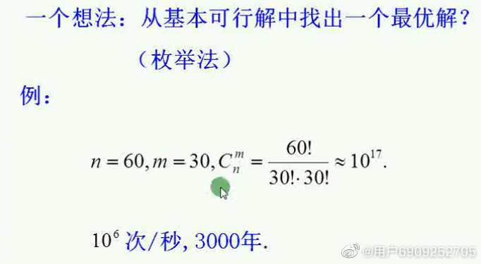
Figure 9 Solution of linear programming
Figure 10 Solution of linear programming
Can you point out the five solutions in the picture above in one step? If it can be pointed out, it will be very specific and not vague. Taking the second example we learned earlier,
It can be known that the feasible solution is the vertex of the feasible domain, and any point in the closed area corresponds to this feasible solution, which is very intuitive;
The basic feasible solution corresponds to the vertices of the feasible region. There are 5 vertices in the feasible region in the coordinate diagram in the above figure, so the basic feasible solutions are these 5 and nothing else.
The optimal solution is all points on the red line segment in the feasible area, and there are infinitely many points.
There are only two basic optimal solutions, which are the two endpoints on the red line segment in the feasible region (also the two vertices of the feasible region); they are not only optimal solutions, but also basic optimal solutions.
There is also a basic solution that does not point out its location, so can it be pointed out from the feasible domain? This one is hard to point out. Because we know before that there is no necessary connection between the basic solution and the feasible solution, and the basic solution is not necessarily a feasible solution.
Feasible solutions are not necessarily basic solutions; that is, feasible solutions are not already basic solutions, so how can you point out which basic solutions are from the feasible domain? But we can find some special basic solutions called basic feasible solutions, because they only have 5 vertices corresponding to them. But we cannot find the general basic solution, because it may not even be a feasible solution.