In this paper, a comparative study of OCV (On-Chip Variation), AOCV (Advanced On-Chip Variation) and POCV (Parameterized On-Chip Variation) is performed. The article also discusses why and how the new mutation model improves over the previous model and performs better with respect to time pessimism.
Introduction:
We have discussed on-chip variations (OCVs) in previous articles. It is recommended to read that article to better understand OCV and its sources. In short, there are two types of process variation:
- Systematic variation (or global variation)
- Random mutation (or local mutation)
Systematic variation has a predictable nature and can be modeled and adjusted as technology nodes mature. But random variation is difficult to model due to its highly unpredictable nature. Systematic variation is handled in PVT, and for random variation we apply a reduction factor to the unit latency. This process variation may change the transistor's current parameters, ultimately affecting the cell's latency. If the cell's latency is affected, it can lead to post-fabrication timing glitches, causing the chip's back-silicon to fail.
To avoid this failure and make the design immune to such process variations, we must keep future process variations in mind and account for expected delay variations when performing static timing analysis (STA).
On-chip variation (OCV):
In OCV, a fixed time reduction factor is applied to the latency of all cells in the design so that if process variation affects the latency of any cell during manufacturing, timing requirements are not affected and the chip does not fail after fabrication.
Variations in the manufacturing process may increase or decrease unit delays. Therefore, when setting the reduction factor, we need to set early and late values. The STA tool will consider early or late timing degradation depending on the path and analysis type. The following is an example of setting the OCV timing reduction factor.
% set_timing_derate -cell_delay-rise -data -early 0.92 % set_timing_derate -cell_delay-rise -data -late 1.10 % set_timing_derate -cell_delay-rise -clock -early 0.95 % set_timing_derate -cell_delay-rise -clock -late 1.06 % set_timing_derate -cell_delay-fall -data -early 0.90 % set_timing_derate -cell_delay-fall -data -late 1.12 % set_timing_derate -cell_delay-fall -clock -early 0.94 % set_timing_derate -cell_delay-fall -clock -late 1.07
In the example above, line 1 sets an early timing reduction factor of 8%, and line 2 sets a late timing reduction factor of 10%, which applies to the rising edge of the data path. Similarly, lines 4 and 5 set the 5% early and 6% late timing reduction factors on the rising edge to the clock path.
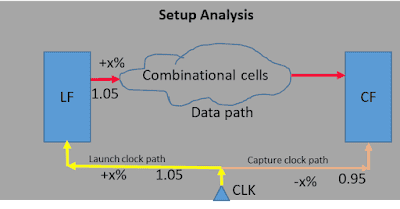
Figure 1 Setting the reduction factor for analysis
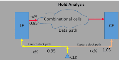
Figure 2 Reduction factors for retention analysis
Figures 1 and 2 show the reduction factors considered by the STA tool in the setup and hold analysis of different paths. In the reg2reg path timing analysis, there is a transmit latch from which the data is emitted and a capture latch that captures the data. The path from the clock source to the clock pin of the transmit latch is called the transmit clock path, and the path from the clock source to the clock pin of the capture latch is called the capture clock path. In setup analysis, the worst-case scenario could be a late data path, a late transmit clock path, and an early capture clock path that could cause setup time failures. Therefore, the STA tool will consider late timing degradation factors for the data path and transmit clock path and early timing degradation factors for the capture clock path.
For holdover analysis, fast data paths, early launch clocks, and late capture clocks are probably the worst case scenarios. Therefore, STA tools always consider the worst case scenario and apply early timing reduction factors to the data path and transmit clock path, and late timing reduction factors to the capture clock path.
Problems in OCV:
In OCV, the fixed time reduction factor used for all units is too pessimistic. In effect, cancellation of the effects of random variation occurs. All units in a particular path may not be all delayed or all advanced. In general, there are always mixed type effects, which lead to a cancellation of the overall effect.
For example, consider a datapath containing 6 buffers with a typical latency of 20ps per cell. Consider late and early reduction factors of 20%. Therefore, assuming all units have later than expected latency, the maximum latency for this path will be 144ps. But in practice, it is rarely the case that all units are only late or only early. It's likely that some will be later and some earlier, so there will be a cancellation of effects and the actual delay will always be less than 144ps. Figure 3 shows the delayed changes in the OCV reduction factor.
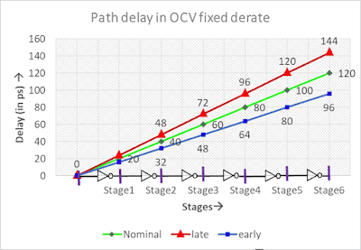
Figure 3 Latency changes with OCV degradation
The concept of OCV fixed reduction factors is modeled in technology nodes above 90nm. This is great for such a higher technology node. But in lower technology nodes, especially in high-frequency designs, timing is more difficult due to the higher pessimism of fixed reduction factors. Therefore, for lower technology nodes, we need to solve this problem. Therefore, the concept of Advanced On-Chip Variation (AOCV) was born, which does not use a fixed reduction factor.
Advanced On-Chip Variation (AOCV):
In AOCV, a reduction factor is applied to each cell based on the path depth and distance of the cell in the timing path, and also varies based on the cell type and the drive strength of the cell. The distance is defined by the mesh and the bounding box of the cell, as shown in Figure 4.
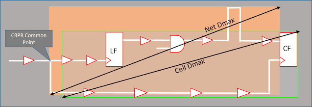
Figure 4 Bounding box of unit and network distance
distance: If the distance increases, the systematic variation increases, and to mitigate this variation we need to use a higher reduction value. So as the distance increases, the reduction value also increases.
path depth: If distance is fixed and path depth increases, systematic variation will remain the same, but random variation will tend to cancel each other out. Therefore, as the path depth increases, the reduction factor will decrease. Figure 5 illustrates path depth in a timing path.
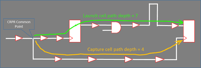
Figure 5 Path depth in the timing path
Unit type: The reduction factor is based on the cell type, e.g. AND gates and OR gates do not exhibit the same variability. The reduction value also varies with the drive strength of the unit, for example AND2X2 and AND2X6 will have different drive reduction values.
AOCV analysis mode:
AOCV supports two analysis modes:
- clock only
- clock and data
In clock-only mode, the AOCV reduction factor is applied only to the clock path, thus reducing effort and improving runtime efficiency. In clock and data mode, the AOCV reduction factor is applied to the entire design. Observing reduced timing pessimism in AOCV, a large number of timing violations have been fixed when we transitioned to clock-only AOCV reduction mode, and violations are further reduced when transitioning to clock and data AOCV mode.
AOCV analysis supports multiple AOCV reduction tables. Two types of tables are generally used, 1D tables or 2D tables. The 1D table contains reduction values that vary with distance or depth, while the AOCV 2D reduction table contains reduction values that vary with both distance and depth. Figure 6 shows an example of an AOCV 2D reduction table.
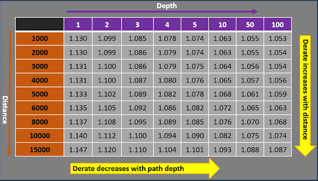
Figure 6 AOCV 2D degradation table example
PrimeTime AOCV process:
Compared to the OCV fixed reduction process, some additional steps are added to the AOCV reduction analysis. The AOCV reduction analysis process of the PrimeTime tool is shown in Figure 7.
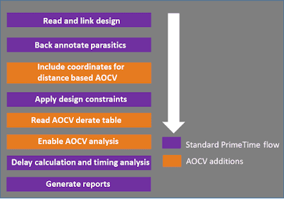
Figure 7 PrimeTime AOCV downgrade process
Problems in AOCV:
AOCV performs poorly below the 40nm technology node, and to improve this we need to further improve timing pessimism. The distance- and depth-based reduction factors used in AOCV are suitable for technology nodes above 40nm, but for nodes below that we need further improvements. To address these issues, parameterized on-chip variation (POCV) was developed. POCV is very effective in 20nm and below technology nodes.
POCV is more realistic than OCV and AOCV. Instead of using distance- and depth-based reduction factors, this method uses delay standard deviation to model the delay variation of cells. The advantage of POCV over AOCV is also that it reduces the relaxed pessimism between graph analysis (GBA) and path analysis (PBA).
Parameterized On-Chip Variation (POCV):
POCV's advanced mutation techniques provide statistical advantages without the need for expensive statistical library characterization. In POCV, instead of applying a specific reduction factor to the cell, the cell delay is calculated based on the cell's delay variation (σ). In POCV, a unit's normal delay values are assumed to follow a normal distribution curve. Figure 8 shows an example of a normal distribution curve and the standard deviation of the data from the mean.
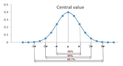
Figure 8 Standard deviation of data from the mean
In a normal distribution, 68% of the data falls within the 1σ range, 95% of the data falls within the 2σ range, and 99.7% of the data falls within the 3σ range.
POCV analysis:
- POCV uses nominal delay values (µ) instead of minimum or maximum values of delays to model random variation.
- Timing analysis is performed in terms of nominal delay values (µ) and delay variation (σ).
- The tool obtains the value of σ from a timing library or an external file containing the POCV coefficient value C.
- Each arc time is then calculated statistically as the sum of nominal delays and variations.
- The tool then calculates the delay of the path by statistically combining these arc delays and performs setup and hold timing analysis.
- By default, the tool performs POCV analysis at 3σ of the mean, but other values can be specified. The larger the standard deviation value, the stronger the temporal pessimism.
POCV input data:
Input for the delay variation σ can be provided to the tool in one of the following ways.
1. Using a single POCV coefficient (C):
An external file containing the delay coefficient value C for each library unit, hierarchy unit, or design. There is only one C value for each timing arc per cell, regardless of input transitions or output loading. The delay variation σ is calculated based on C as follows.
POCV coefficient file example:
ocvm_type: pocvm
object_type: lib_cell
rf_type: rise fall
delay_type: cell
derate_type: early
object_spec: */INV*
coefficient: 0.0693
2. Use Library Variation Format (LVF):
Information on POCV variants is provided directly to the library in LVF format. In LVF format, there are two indexes, one for the input transition and another for the output load. An example of POCV LVF format is shown below.
sigma_type : “late”; index_1(“0.01, 0.04, 0.12, 0.80”); index_2(“0.01, 0.02, 0.03, 0.10”); values( “σ11, σ12, σ13, σ14”, “σ21, σ22, σ23, σ24”, “σ31, σ32, σ33, σ34”, “σ41, σ42, σ43, σ44”, ); }
Typically, index-1 represents the input transition and index-2 represents the output load. If both data types are present in the design, a single POCV coefficient file takes precedence by default over a POCV slew-load table or LVF format file.
POCV delay calculation:
Among them
C = POCV coefficient
N = number of standard deviations
or
PrimeTime POCV analysis process:
The process used by the PrimeTime tool for POCV reduction analysis is shown in Figure 9.
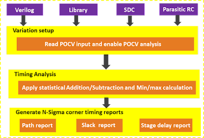
Figure 9 PrimeTime POCV analysis process
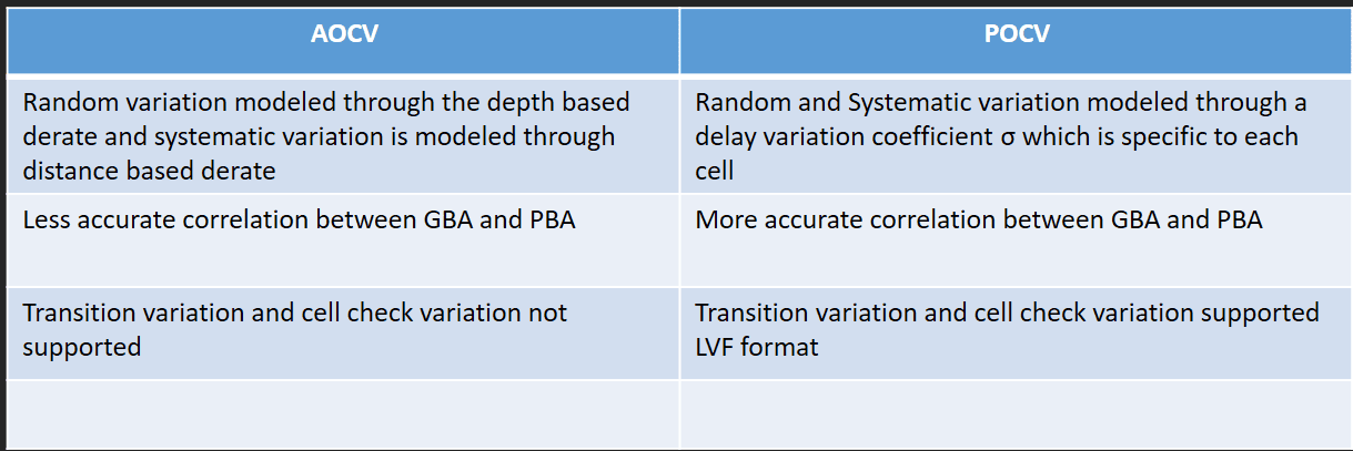
Comparison of POCV and AOCV:
Here is a basic comparison between POCV and AOCV:
thank you
[1] https://teamvlsi.com/2020/07/ocv-aocv-and-pocv-in-vlsi-comparative.html